Tutorial 1: Amplicon prepared with RT-PCR
This tutorial demonstrates how to analyze a dataset that was prepared using RT-PCR (with forward and reverse primers) of one specific region of an RNA.
TL;DR
Un-tar and enter the data directory:
tar xvf data.tar
cd data
Process the no-DMS control:
seismic wf -x fq/nodms --keep-g --keep-u --mask-polya 0 --min-mut-gap 0 hiv-rre.fa
Process the DMS-treated replicates separately:
seismic wf -x fq/dms1 -x fq/dms2 --mask-pos rre 176 -P rre GGAGCTTTGTTCCTTGGGTTCTTGG GGAGCTGTTGATCCTTTAGGTATCTTTC hiv-rre.fa
seismic graph scatter out/dms[12]/filter/rre/26-204/filter-position-table.csv
Pool the replicates and process them together:
seismic pool dms-pool out/dms[12]
seismic wf --mask-pos rre 176 -P rre GGAGCTTTGTTCCTTGGGTTCTTGG GGAGCTGTTGATCCTTTAGGTATCTTTC -k 2 --fold --fold-quantile 0.95 hiv-rre.fa out/dms-pool/idmut
Scientific premise
The RNA in this example is a segment of the the human immunodeficiency virus 1 (HIV-1) genome called the Rev response element (RRE), which binds to the protein Rev that mediates nuclear export (Sherpa et al.). The RRE RNA folds into two different secondary structures: a predominant (~75%) structure with 5 stems and a minor (~25%) structure with 4 stems, each of which is associated with a different rate of HIV-1 replication.
In this hypothetical experiment, you in vitro transcribe a 232 nt segment of the RRE, perform two DMS-MaPseq experiments on it (along with a no-DMS control), amplify a region using RT-PCR, and sequence the amplicons using paired-end 150 x 150 nt read lengths.
The FASTQ files in this tutorial were actually generated using seismic sim
and don’t resemble the authentic DMS mutational patterns.
Download example files of an amplicon
Download the example FASTA and FASTQ files. First, open your terminal and navigate to a directory in which you want to run the tutorial.
If you have wget, you can download the tutorial data simply by typing
wget https://raw.githubusercontent.com/rouskinlab/seismic-rna/main/src/userdocs/tutorials/amplicon/data.tar
Otherwise, click this link to download the tutorial data: https://raw.githubusercontent.com/rouskinlab/seismic-rna/main/src/userdocs/tutorials/amplicon/data.tar
To ensure the download is complete and not corrupted, verify that the SHA-256
checksum is 00c500bc9458048af04ee09b397a59e829fa25c7a53ba6c1b5cc09cbf80cd6ee
by typing this command:
shasum -a 256 data.tar
If this command prints a different checksum, then retry the download. If the problem persists, then raise an issue (see Bugs and Requests).
After downloading and verifying the data, untar the data by typing
tar xvf data.tar
and then navigate into the data directory:
cd data
Process the no-DMS control
When you have a no-DMS control, it is a good idea to analyze it first to check if any bases are highly mutated: such bases would give falsely high mutation rates and should be ignored while analyzing DMS-modified samples.
Run the workflow on the no-DMS control
Process the no-DMS control through the whole workflow with this command:
seismic wf -x fq/nodms --keep-g --keep-u --mask-polya 0 --min-mut-gap 0 hiv-rre.fa
This is what each of the arguments does:
wfmeans run the entire workflow.-x fq/nodmsmeans search insidefq/nodmsfor pairs of FASTQ files of paired-end reads with mate 1 and mate 2 in separate files.--keep-g --keep-umeans keep G and U bases (which do not react with DMS and should typically be masked out in DMS-modified samples).--mask-polya 0means do not mask out poly(A) sequences (which can produce artifacts in DMS-modified samples).--min-mut-gap 0means disable observer bias correction (which only appies to DMS-modified samples).hiv-rre.fameans use the sequence in this FASTA file as the reference (i.e. mutation-free) sequence for the RNA.
After it finishes running (which should take about one minute or less), all
output files will go into the directory out.
Check the graphs of coverage and mutation rate for the no-DMS control
Next, check the unambiguous count (i.e. how many base calls at each position
could be labeled unambiguously as either a match or a mutation).
Open out/nodms/graph/rre/full/profile_filtered_n-count.html in a web broser.
nodmsis the samplerreis the reference (i.e. name of the RNA)fullis the region of the reference you are looking atprofileis the type of graph (a bar graph with position on the x-axis)filteredmeans graph the data come from the Filter stepnis the shorthand for “unambiguous”countmeans graph the number of reads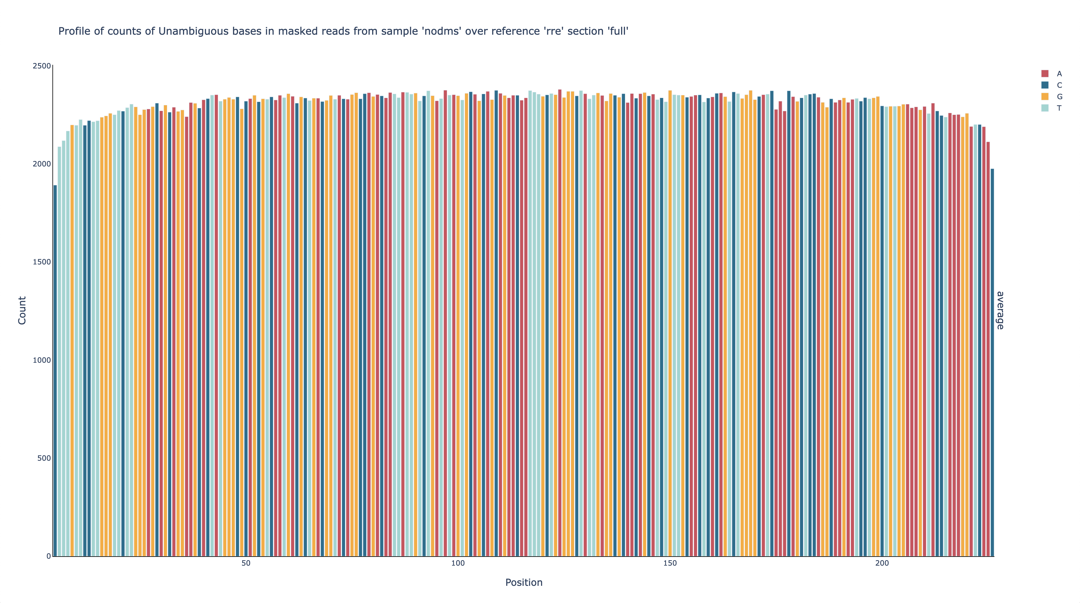
This graph shows that the number of unambiguous base calls at each position is fairly even – around 2,200 – across all positions amplified by the primers (56-222), which is expected for RT-PCR amplicons. This graph also shows that each position has enough unambigous base calls (>1,000) to obtain a reasonably accurate estimate of the mutation rate.
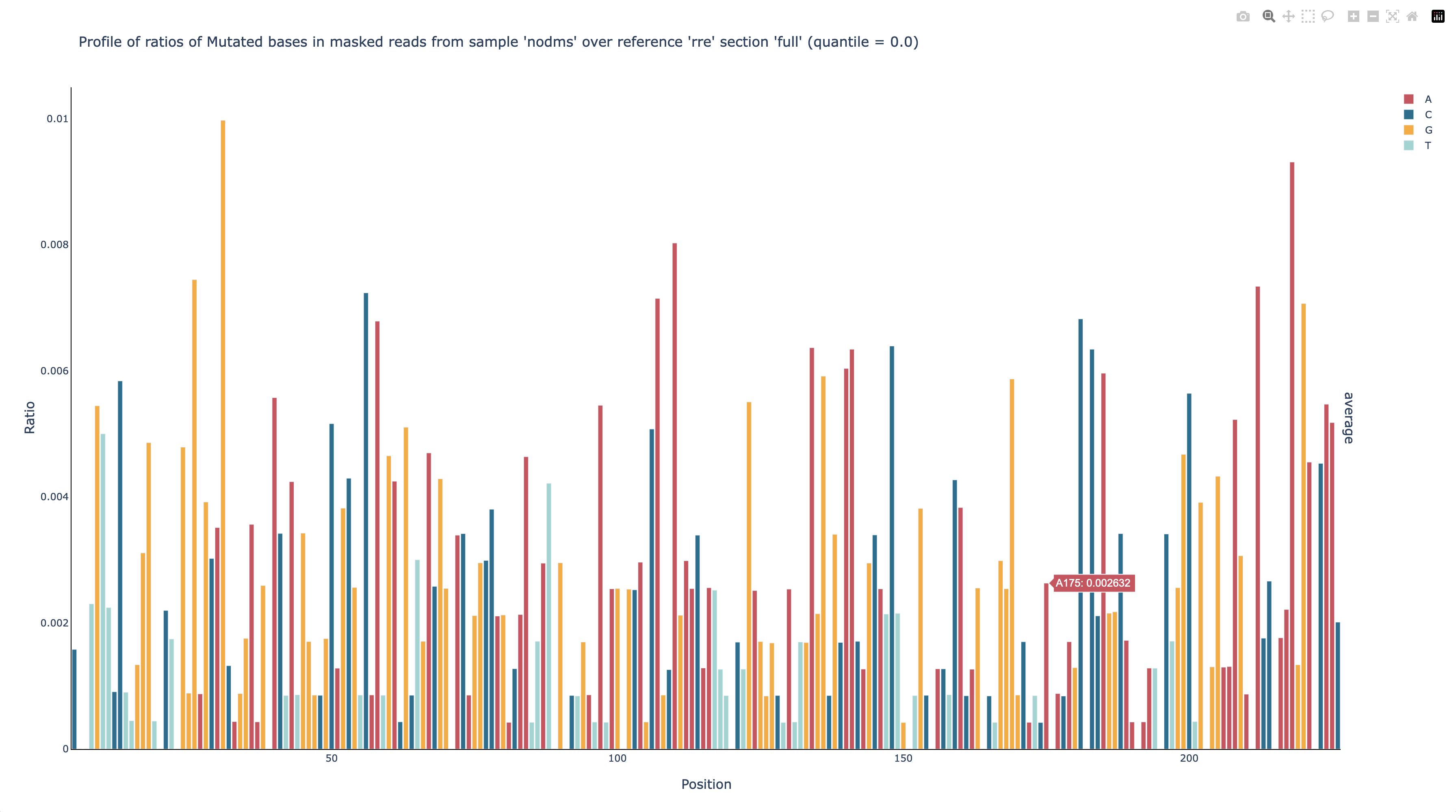
After confirming there are sufficient unambiguous base calls, view the mutation
rates by opening out/nodms/graph/rre/full/profile_filtered_m-ratio-q0.html
in a web browser.
nodms,rre,full,profile, andfilteredhave the same meanings as beforemis the shorthand for “mutated”ratiomeans graph the ratio ofm(mutated) to unambiguously mutated or matching base calls (i.e. the mutation rate)q0means do not normalize the mutation rates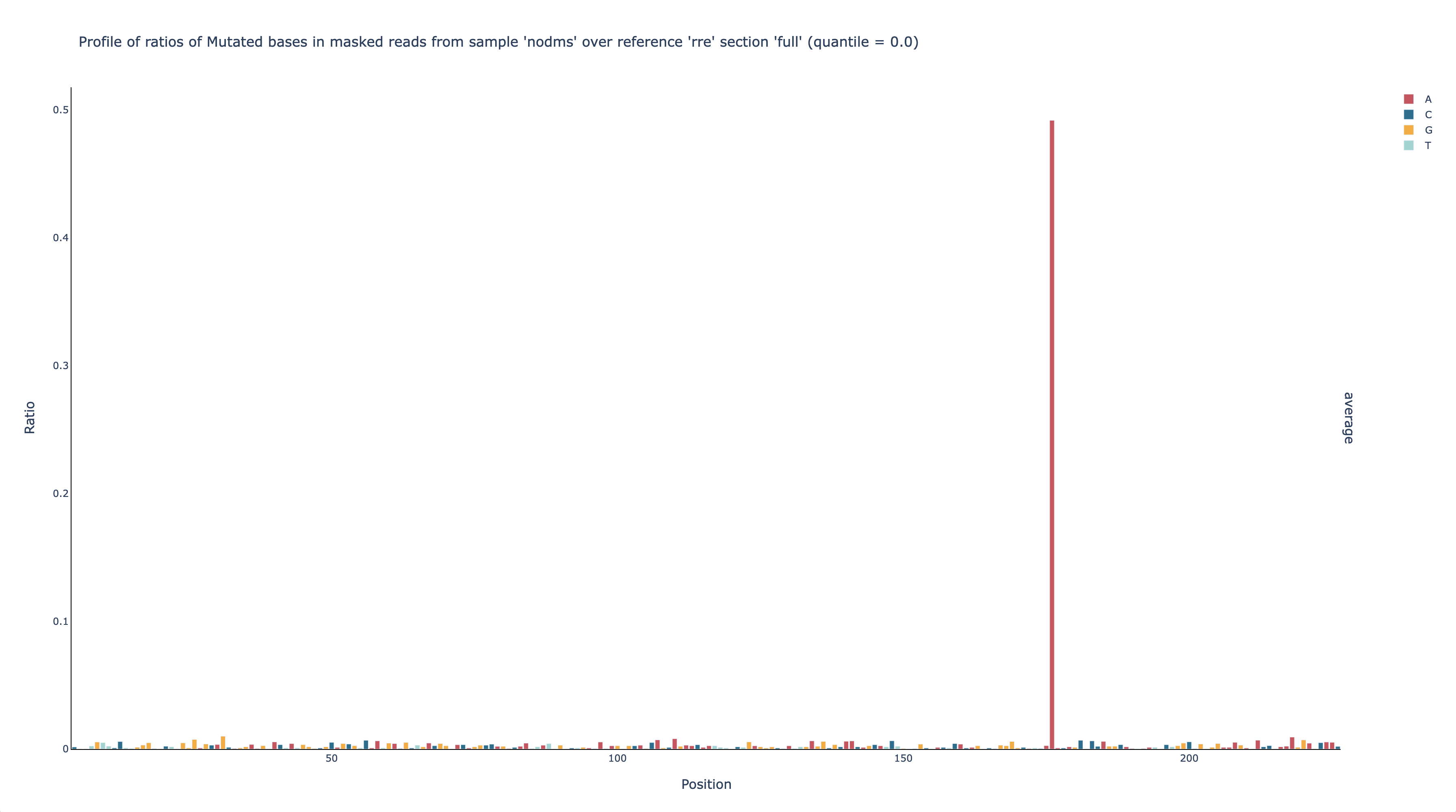
This graph shows that the mutation rate is very low across all positions – as expected for a sample that is not DMS-modified – except for position 176, which has a mutation rate of nearly 50%. Because of this one outlier, it is hard to see just how low the mutation rates are at the other positions, but because this graph is interactive, you can click at the top of the y-axis and enter a new upper limit, such as 0.02. You can also mouse over a bar to see its mutation rate (G31 is shown here).
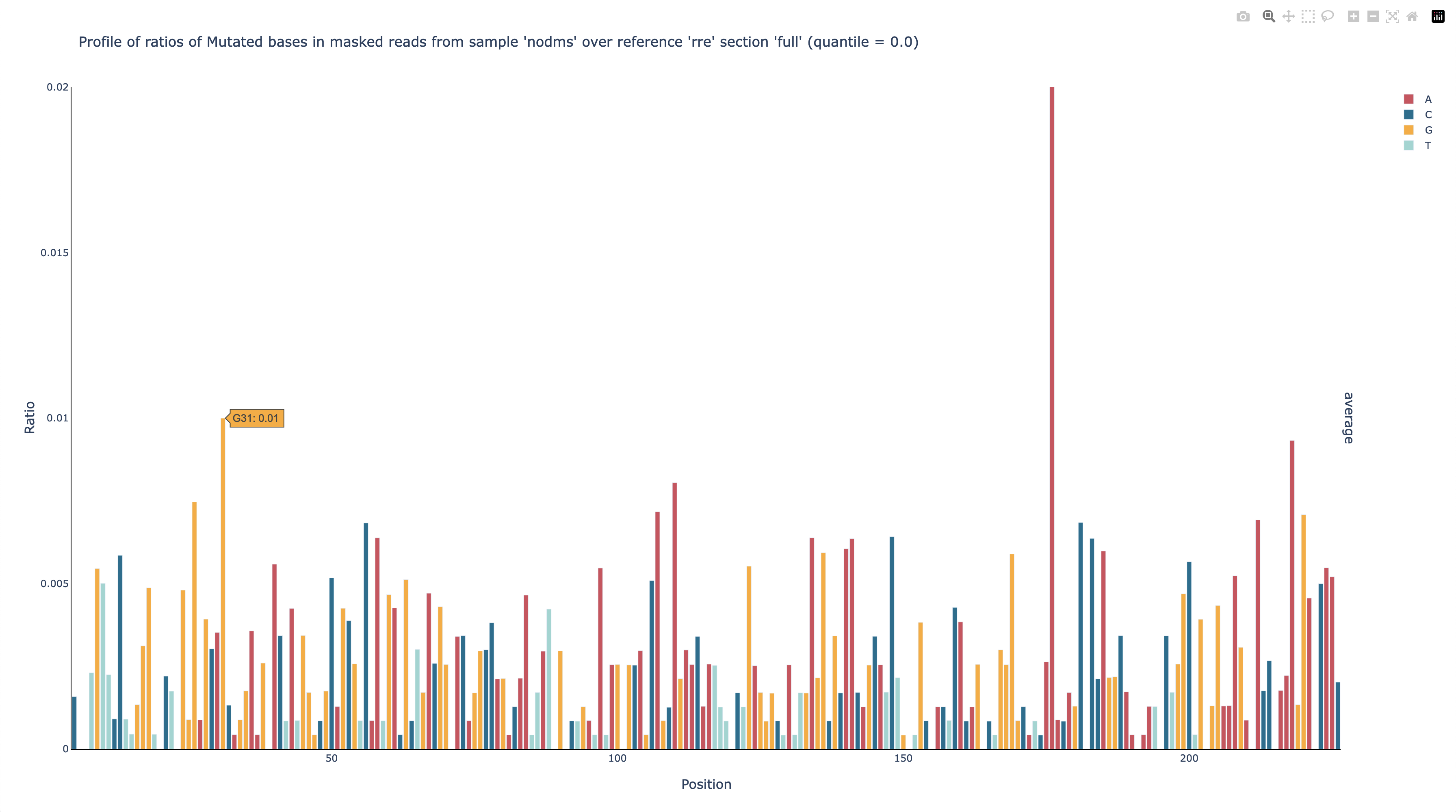
Now it is clear that every position except 176 has a mutation rate no greater than 1%, and most are below 0.5%, which is typical for non-DMS-modified RNA.
To figure out why position 176 has such a high mutation rate, you can check the
types of mutations that occur at each position, which are in another graph,
out/nodms/graph/rre/full/profile_filtered_acgtdi-ratio-q0.html.
nodms,rre,full,profile,filtered,ratio, andq0have the same meanings as beforeacgtdiare the shorthands for substitutions to A, C, G, and T; deletions; and insertions; respectively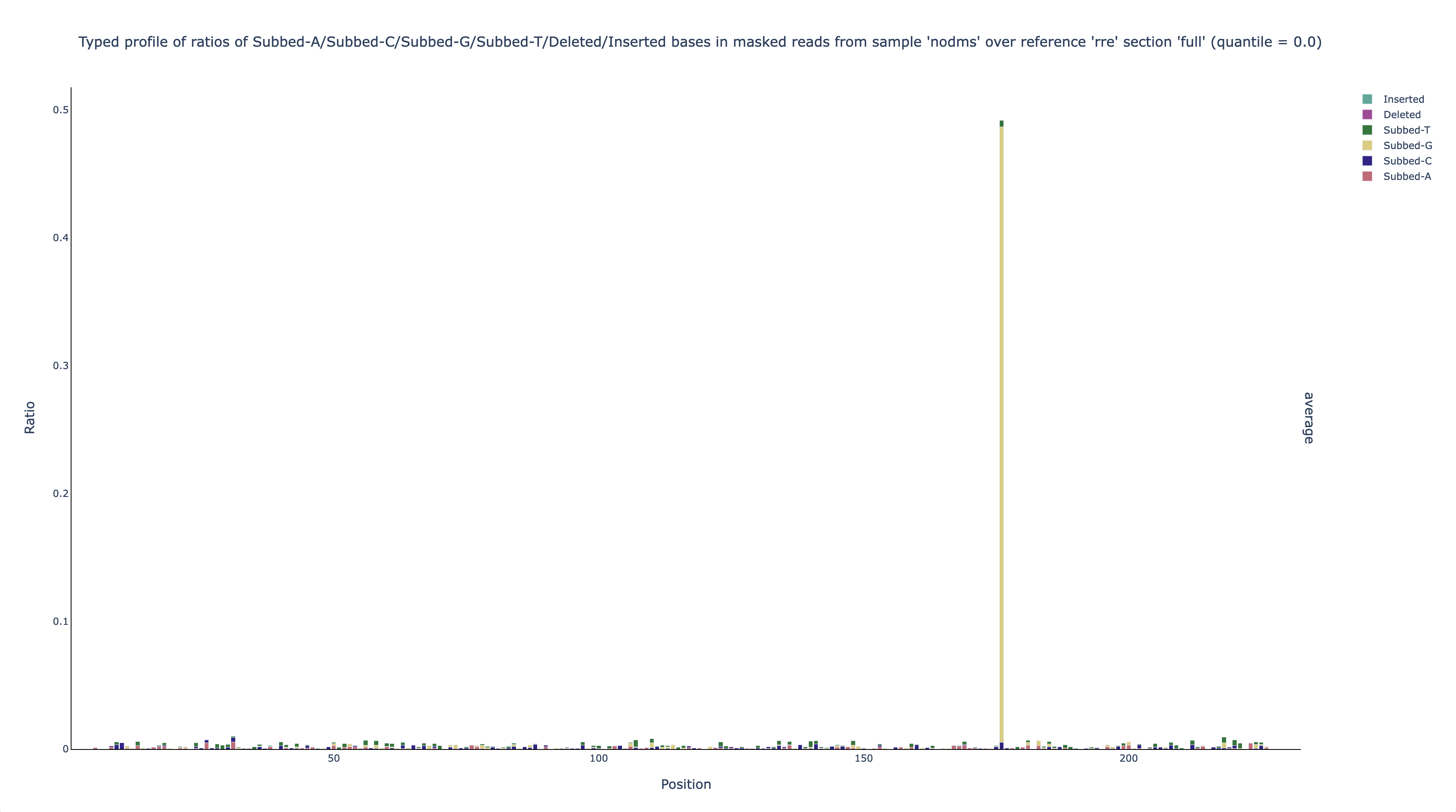
This graph shows that nearly all (~97%) of the mutations at position 176 are A-to-G substitutions. This finding suggests (given that this hypothetical experiment is in vitro) that the DNA template that was used to transcribe the RNA could actually be a mixture of about 50% the expected sequence and 50% that sequence with an A-to-G substitution at position 176.
Mask out the position that is highly mutated in the no-DMS sample
If this were a real experiment, it could be worth sequencing the DNA template to check if it actually was a mixture, and if so to fix it. For the purposes of this tutorial, you will learn how to mask out position 176 so that it does not skew the results.
Rerun the workflow with the option --mask-pos rre 176:
seismic wf --force --keep-g --keep-u --mask-polya 0 --min-mut-gap 0 --mask-pos rre 176 hiv-rre.fa out/nodms/idmut/rre
This is what each of the arguments does:
wfmeans run the entire workflow.--forcemeans overwrite any output files that already exist.--keep-g --keep-umeans keep G and U bases (which do not react with DMS and should typically be masked out in DMS-modified samples).--mask-polya 0means do not mask out poly(A) sequences (which can produce artifacts in DMS-modified samples).--min-mut-gap 0means disable observer bias correction (which only appies to DMS-modified samples).--mask-pos rre 176means mask position 176 in referencerre.hiv-rre.fameans use the sequence in this FASTA file as the reference (i.e. mutation-free) sequence for the RNA.out/nodms/idmut/rremeans search this directory for data files: in this case, the data from the IDmut step for samplenodms, referencerre.
After the command finishes running, you can see that position 176 was masked out
by opening out/nodms/graph/rre/full/profile_filtered_m-ratio-q0.html (position
175 is highlighted to make the gap between it and position 177 more clear):
Process both DMS-modified replicates
Now you are ready to process the DMS-modified samples.
Run the workflow on both DMS-treated replicates
Process the DMS-treated samples through the whole workflow with this command:
seismic wf -x fq/dms1 -x fq/dms2 --mask-pos rre 176 -P rre GGAGCTTTGTTCCTTGGGTTCTTGG GGAGCTGTTGATCCTTTAGGTATCTTTC hiv-rre.fa
This is what each of the arguments does:
wfmeans run the entire workflow.-x fq/dms1means search insidefq/dms1for pairs of FASTQ files of paired-end reads with mate 1 and mate 2 in separate files.-x fq/dms2means search insidefq/dms2for pairs of FASTQ files of paired-end reads with mate 1 and mate 2 in separate files.--mask-pos rre 176means mask position 176 (because it had a high mutation rate in the no-DMS sample).-P rre GGAGCTTTGTTCCTTGGGTTCTTGG GGAGCTGTTGATCCTTTAGGTATCTTTCdefines a region of the referencerrethat corresponds to the amplicon flanked by primersGGAGCTTTGTTCCTTGGGTTCTTGGandGGAGCTGTTGATCCTTTAGGTATCTTTC.hiv-rre.fameans use the sequence in this FASTA file as the reference (i.e. mutation-free) sequence for the RNA.
Check the correlation of mutation rates between DMS-treated replicates
Next, it is recommended to check the correlation of mutation rates between the replicates, to ensure they are reproducible. To create a scatter plot of the mutation rates and calculate the correlation, run the command
seismic graph scatter out/dms[12]/filter/rre/26-204/filter-position-table.csv
graph scattermeans graph a scatter plot.out/dms[12]/filter/rre/26-204/filter-position-table.csvmeans graph data from these tables, where[12]is a glob pattern that is expanded by the shell into all files that match the pattern – which in this case isout/dms1/filter/rre/26-204/filter-position-table.csv out/dms2/filter/rre/26-204/filter-position-table.csv. You could instead type this expression to list both table files explicitly, but the former requires fewer key strokes.
Open out/dms1__and__dms2/graph/rre/26-204/scatter_filtered_m-ratio-q0.html
in a web browser to view the scatter plot and correlation:
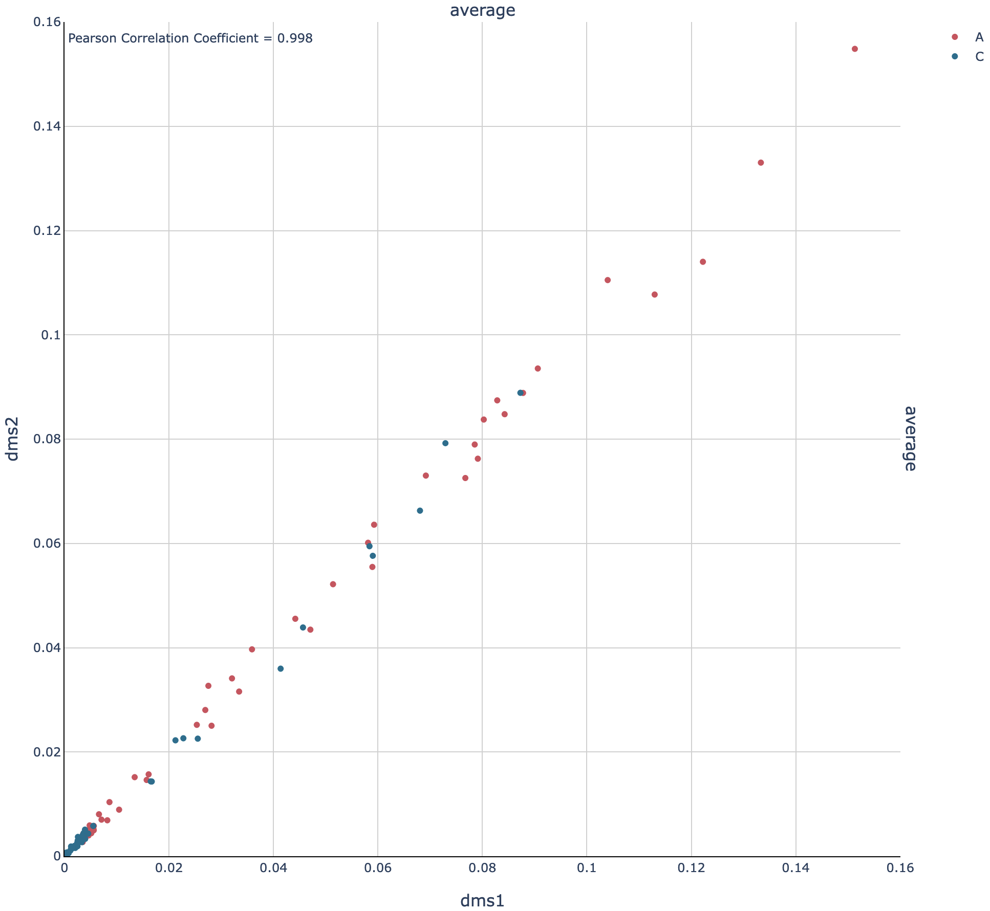
The Pearson correlation is 0.998, which is extremely high. (For a general amplicon, ≥0.98 would be ideal, and ≥0.95 would be decent).
Pool the DMS-treated replicates and process them together
Pool the two DMS-treated replicates
Because the correlation is so high, the data from the replicates can be combined so that they can be analyzed as a single sample, which is helpful whenever high coverage is necessary, such as during clustering. To combine the replicates, run this command:
seismic pool dms-pool out/dms[12]
poolmeans combine samples into a new “pooled” sample.dms-poolmeans name the pooled sampledms-pool.out/dms[12]means pool the samples in these directories, where[12]is a glob pattern that is automatically expanded by the shell into all files that match the pattern – which in this case isout/dms1 out/dms2. You could instead type this expression to list both table files explicitly, but the former requires fewer key strokes.
Process the pooled DMS-treated samples
Now that the replicates are pooled, the overall coverage will be higher, and so clustering is more likely to detect true alternative structures. Process the pooled sample, including with clustering, by running this command:
seismic -v wf --mask-pos rre 176 -P rre GGAGCTTTGTTCCTTGGGTTCTTGG GGAGCTGTTGATCCTTTAGGTATCTTTC -k 2 --fold --fold-quantile 0.95 hiv-rre.fa out/dms-pool/idmut
This is what each of the arguments does:
-vmeans use verbose mode (to print more messages to the console).wfmeans run the entire workflow.--mask-pos rre 176means mask position 176 (because it had a high mutation rate in the no-DMS sample).-P rre GGAGCTTTGTTCCTTGGGTTCTTGG GGAGCTGTTGATCCTTTAGGTATCTTTCdefines a region of the referencerrethat corresponds to the amplicon flanked by primersGGAGCTTTGTTCCTTGGGTTCTTGGandGGAGCTGTTGATCCTTTAGGTATCTTTC.-k 2means enable clustering to find alternative structures.--foldmeans enable secondary structure prediction.--fold-quantile 0.95sets the 95th percentile of the mutation rates to 1 and scales the rest of the data accordingly (optional; 0.95 is the default).hiv-rre.fameans use the sequence in this FASTA file as the reference (i.e. mutation-free) sequence for the RNA.out/dms-pool/idmutmeans search insideout/dms-pool/idmutfor data to feed into the workflow: in this case, a report from the IDmut step.
Check whether the RNA forms alternative structures
To check whether alternative structures were detected, open the cluster report
in a web browser: out/dms-pool/cluster/rre/26-204/cluster-report.json.
The contents of the report will resemble this (some fields may differ, such as
the time and version):
{
    "Sample": "dms-pool",
    "Branches": {
        "align": "",
        "idmut": "",
        "filter": "",
        "cluster": ""
    },
    "Reference": "rre",
    "Region": "26-204",
    "Seed for the random number generator": 708453219,
    "Start at this many clusters": 1,
    "Stop at this many clusters (0 for no limit)": 2,
    "Try all numbers of clusters (Ks), even after finding the best number": false,
    "Write all numbers of clusters (Ks), rather than only the best number": false,
    "Remove runs with two clusters more similar than this correlation": 0.9,
    "Remove runs with two clusters that differ by less than this MARCD": 0.016,
    "Remove runs where a cluster differs by more than this ARCD from the ensemble average at any position": 0.2,
    "Remove runs where any cluster's Gini coefficient exceeds this limit": 0.667,
    "Calculate the jackpotting quotient to find over-represented reads": true,
    "Confidence level for the jackpotting quotient confidence interval": 0.95,
    "Remove runs whose jackpotting quotient exceeds this limit": 1.1,
    "Maximum number of simulations to compute the jackpotting quotient": 12,
    "Skip calculating the jackpotting quotient if the reads × positions exceeds this limit": 268435456,
    "Remove Ks with a log likelihood gap larger than this (0 for no limit)": 0.0,
    "Remove Ks where every run has less than this correlation vs. the best": 0.97,
    "Remove Ks where every run has more than this MARCD vs. the best": 0.008,
    "Run EM (successfully) at least this number of times for each K": 6,
    "Run EM (successfully or not) at most this number of times for each K": 30,
    "Run EM for at least this many iterations": 10,
    "Run EM for at most this many iterations": 500,
    "Stop EM when the log likelihood increases by less than this threshold": 0.37,
    "Number of unique reads": 12236,
    "Whether each number of clusters (K) passed filters": {
        "1": true,
        "2": true
    },
    "Best number of clusters": 2,
    "Numbers of clusters written to batches": [
        2
    ],
    "Number of batches": 2,
    "Checksums of batches (SHA-512)": {
        "cluster": [
            "8f42feceefca3aba6dfbf2fba8072ecf7b1d6b1a9e3c0d5f4a2b8c7d6e5f40312a9b8c7d6e5f4039281706a5b4c3d2e1f0a9b8c7d6e5f4039281706a5b4c3d2e1",
            "f3bb0d2bdd105ec91c3f84bf3a194bfe2c0d5f4a2b8c7d6e5f40312a9b8c7d6e5f4039281706a5b4c3d2e1f0a9b8c7d6e5f4039281706a5b4c3d2e1f0a9b8c7d6"
        ]
    },
    "Time began": "2024-12-08 at 23:10:31",
    "Time ended": "2024-12-08 at 23:12:16",
    "Time taken (minutes)": 1.75,
    "Version of SEISMIC-RNA": "0.25.3"
}
The number of clusters detected is the field Best number of clusters, which
is 2 in this case, suggesting that the RNA forms 2 alternative structures.
Draw the best-supported structure model for each cluster
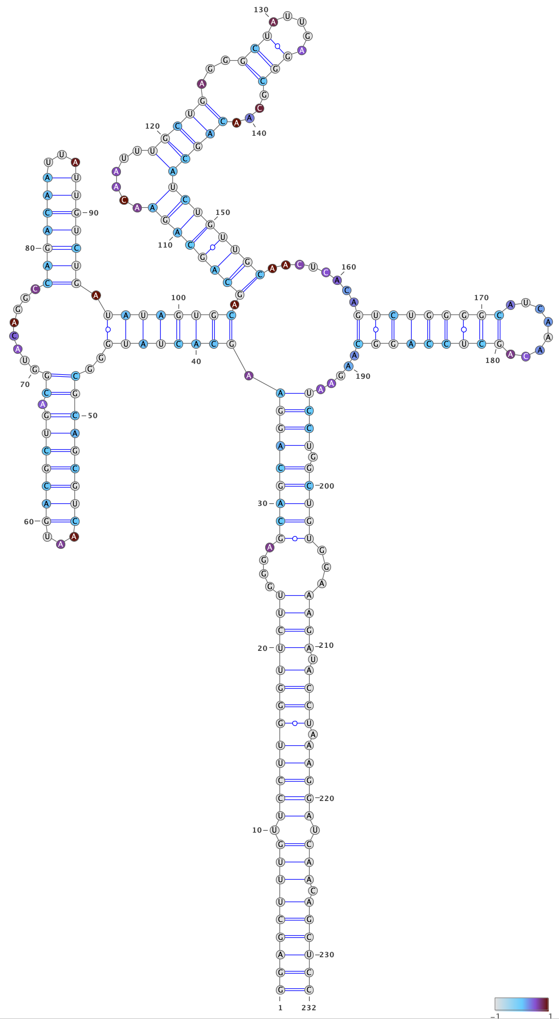
For each cluster, the DMS reactivities are used to model the secondary structure
of the RNA (with the --fold option).
However, the folding algorithm will produce a structure for any DMS reactivties
– even pure noise.
Thus, it is important to verify that the structure models agree with the DMS
reactivities – that is, paired bases tend to have low reactivities and unpaired
bases tend to have high reactivities.
The agreement is measured by computing the receiver operating characteristic (ROC) and calculating the area under the curve (AUC). If the structure agrees perfectly with the DMS reactivities – that is, every unpaired base has a higher DMS reactivity than every paired base – then the AUC will equal 1. If the DMS reactivities were completely random, then the AUC would be 0.5.
Open out/dms-pool/graph/rre/full/roc_26-204__clustered-2-x_m-ratio-q0.html
in a web browser to check the AUC-ROC for this sample.
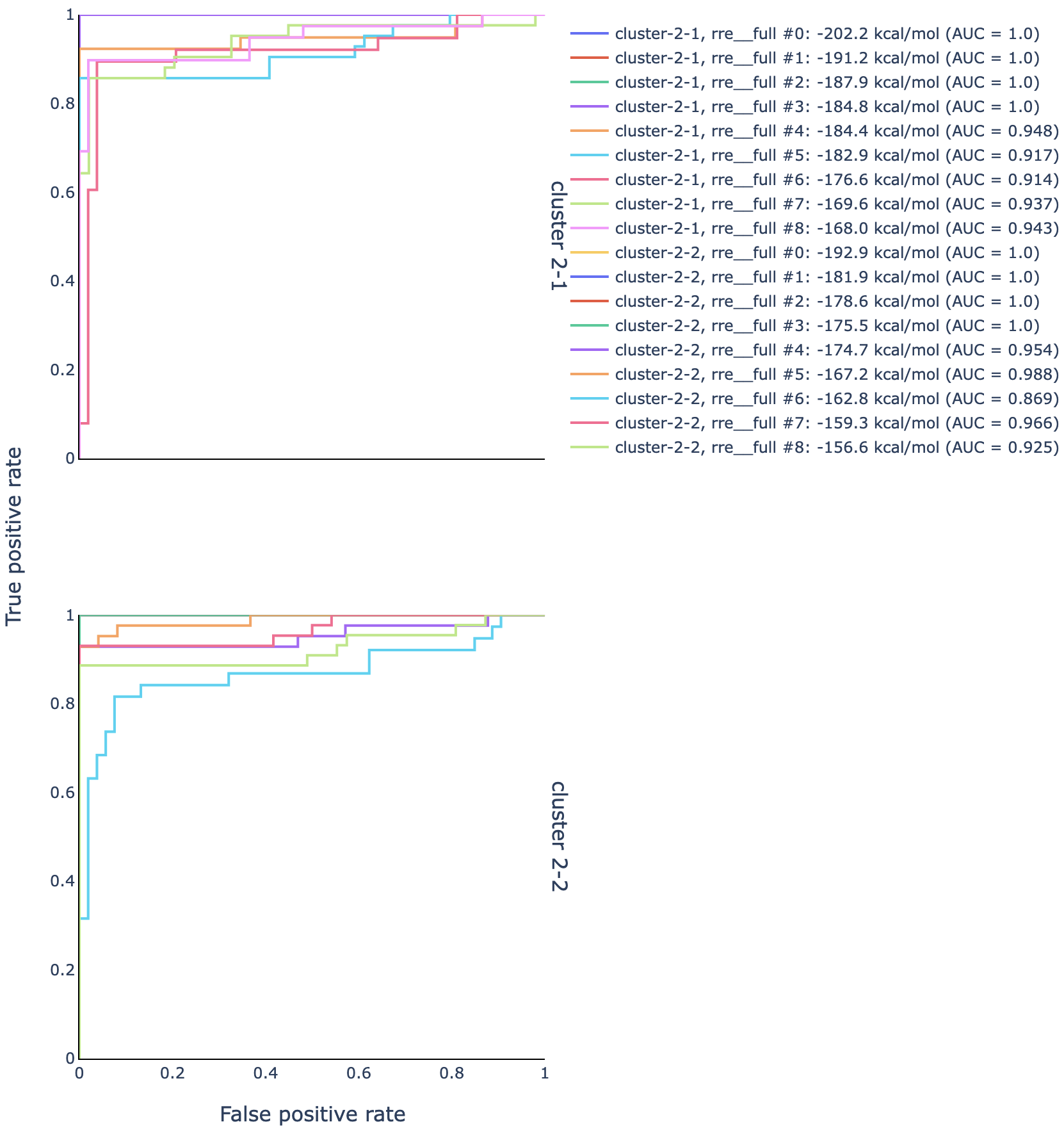
The ROC curves for structures modeled using the DMS reactivities from cluster 1
are in the upper graph, and those from cluster 2 in the lower graph.
For each cluster, multiple structures were modeled: generally, the best model is
the one with the largest AUC, and if there is a tie for the largest AUC, then
the model among those with the smallest (most negative) free energy.
In this case, that is structure rre__full #0 for both clusters.
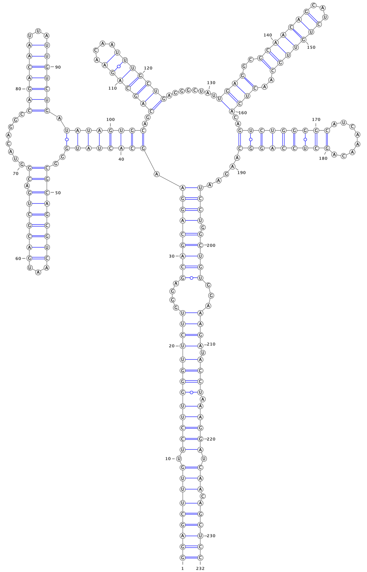
In a text editor, open the structure models for cluster 1:
out/dms-pool/fold/rre/full/26-204__cluster-2-1.db
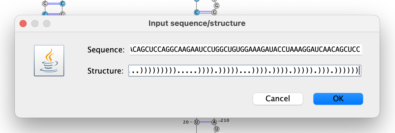
Copy the sequence (second line) as well as the structure on the line below
rre__full #0 into an RNA structure visualization program, such as VARNA.
Adjust the angles to remove overlaps between different parts of the structure.
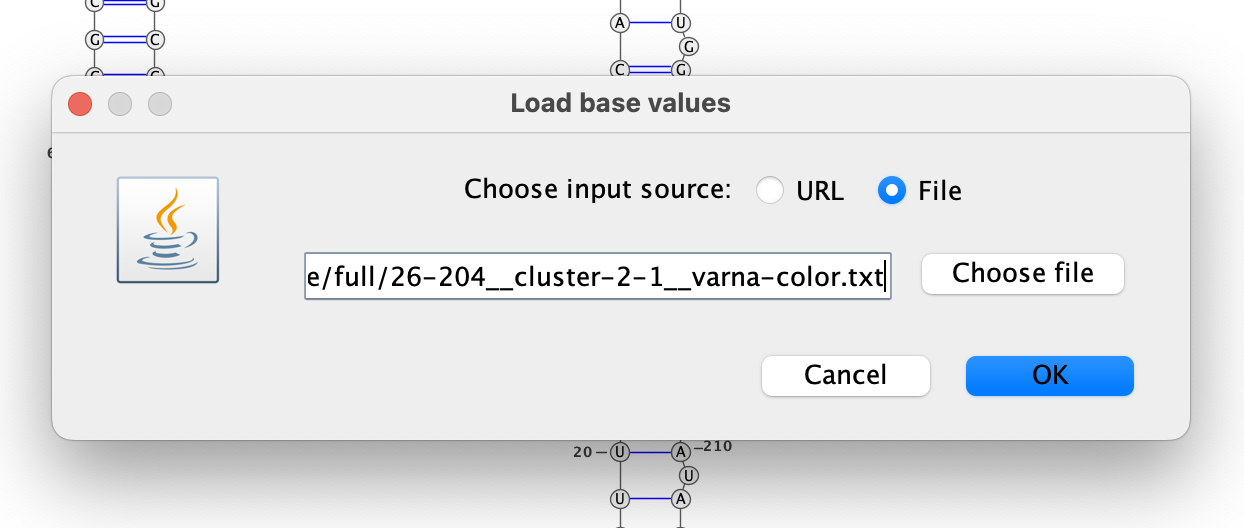
Color the bases by their DMS reactivities by right-clicking on the VARNA canvas,
choosing “Color map” then “Load values…”, and then typing the VARNA color file
out/dms-pool/fold/rre/full/26-204__cluster-2-1__varna-color.txt in the box.
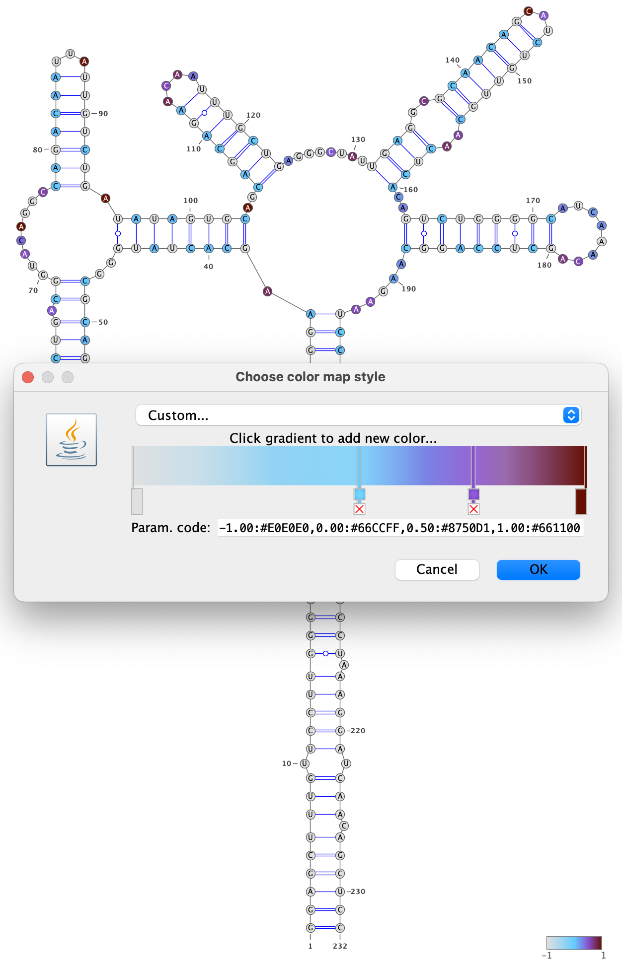
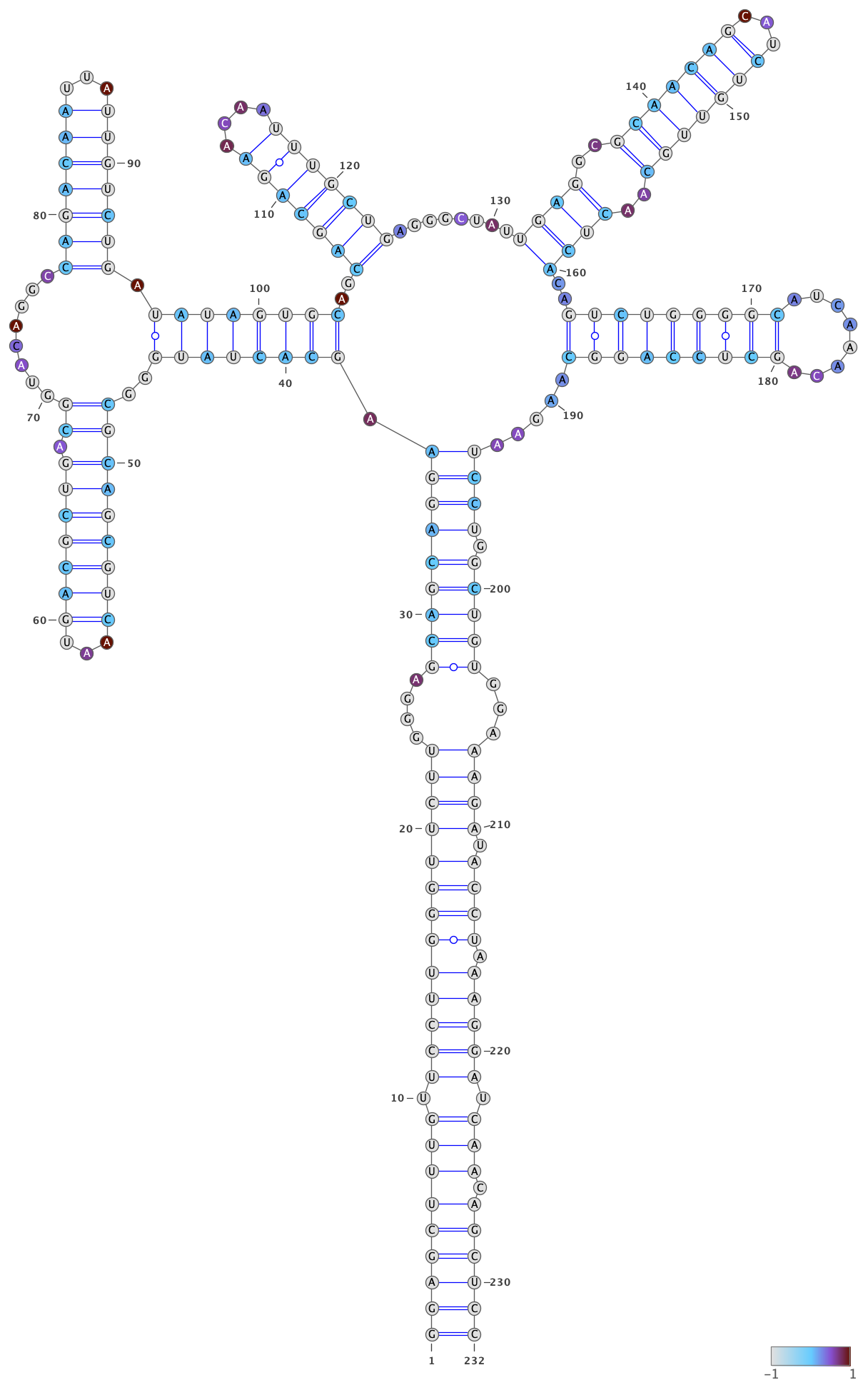
Specify a color palette by right-clicking on the VARNA canvas, choosing “Color map” and then “Style…”. Bases with no data are set to -1, and bases with data are set to a value between 0 and 1, so choose a color palette that is consistent with this scheme, such as light gray for -1 and a gradient from 0 to 1:
Save the VARNA session file by right-clicking on the VARNA canvas, choosing “Save…”, selecting “VARNA Session File” under “File Format”, and entering a location and name for the file.
To draw the structure for cluster 2, right-click the VARNA canvas, choose
“New…”, open out/dms-pool/fold/rre/full/26-204__cluster-2-2.db in a text
editor, and copy-paste the structure below rre__full #0 into the text box
“Structure.”
Repeat the steps above to draw and color the structure for cluster 2, except
using out/dms-pool/fold/rre/full/26-204__cluster-2-2__varna-color.txt as the
source of the DMS reactivities for the colors.